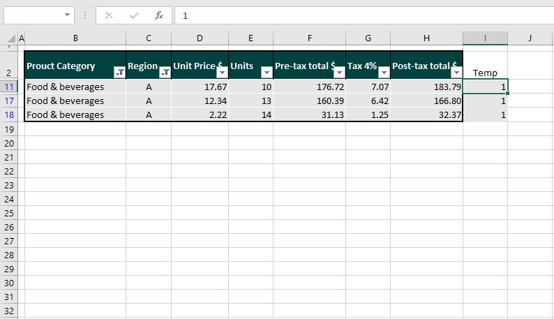
Excel’s filtering feature is a powerful tool that allows you to quickly identify and focus on relevant data within your spreadsheet. However, once you’ve applied a filter, the hidden rows can still consume valuable space and make your document appear cluttered. In this comprehensive guide, we’ll walk you through the process of deleting filtered rows in Excel, empowering you to maintain a clean and organized spreadsheet.
Understanding the Importance of Deleting Filtered Rows
Deleting filtered rows in Excel serves several key purposes:
- Improved Readability and Navigation: Removing unnecessary filtered rows can make your spreadsheet more concise and easier to navigate, allowing you and your team to focus on the relevant data without distractions.
- Enhanced Data Analysis and Visualization: Eliminating filtered rows can ensure that your data is presented in a more streamlined and coherent manner, making it easier to perform calculations, create charts, and generate meaningful insights.
- Optimized Storage and Performance: Excessively large Excel files with many hidden rows can slow down your computer’s performance and consume more storage space. Deleting these rows can help optimize the file size and enhance the overall efficiency of your spreadsheet.

How to Delete Filtered Rows in Excel: Step-by-Step Guide
Now, let’s explore the step-by-step process of deleting filtered rows in Excel:
Step 1: Apply a Filter to Your Data
Begin by applying a filter to your Excel data. You can do this by selecting the entire range of data and then clicking the “Filter” button on the “Data” tab in the Excel ribbon.
Step 2: Identify the Filtered Rows
After applying the filter, you’ll notice that some rows in your spreadsheet are now hidden. These are the filtered rows that you can choose to delete.
Step 3: Delete the Filtered Rows
To delete the filtered rows, follow these steps:
- Make sure the filter is still active on your data.
- Right-click on any of the visible row numbers (the ones that aren’t hidden).
- In the context menu, select the “Delete” option.
- Excel will now delete all the filtered rows, leaving only the visible rows in your spreadsheet.
Step 4: Remove the Filter (Optional)
After deleting the filtered rows, you may want to remove the filter from your spreadsheet to restore the full dataset. To do this, simply click the “Filter” button on the “Data” tab again to turn off the filter.
Step 5: Regularly Review and Maintain
Deleting filtered rows in Excel should be a regular part of your spreadsheet maintenance routine. Make it a habit to review your data, apply filters as needed, and delete any unnecessary filtered rows to keep your Excel document clean and efficient.
Conclusion: Embracing a Clutter-Free Excel Experience
Deleting filtered rows in Excel is a valuable skill that can help you maintain a well-organized and efficient spreadsheet environment. By following the steps outlined in this guide, you can quickly identify and remove unwanted filtered rows, improving the overall readability, data analysis, and performance of your Excel documents.
Remember, regular maintenance and optimization of your Excel spreadsheets can have a significant impact on your productivity and the quality of your data. Embrace the power of filtered row deletion, and let the benefits of a decluttered Excel experience transform your data management workflows.


Add Comment